Eigen values and vectors

Definition

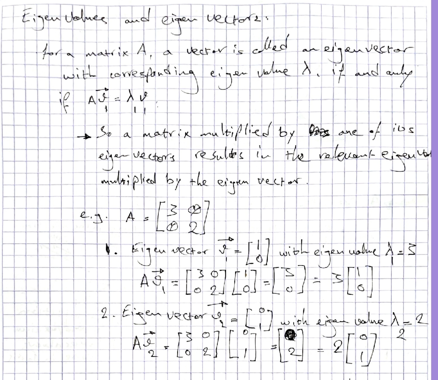
For a square matrix A, a scalar λ is an eigenvalue of A if there exists a non-zero vector v such that:

Av = λv

The non-zero vector v is called an eigenvector corresponding to the eigenvalue λ.

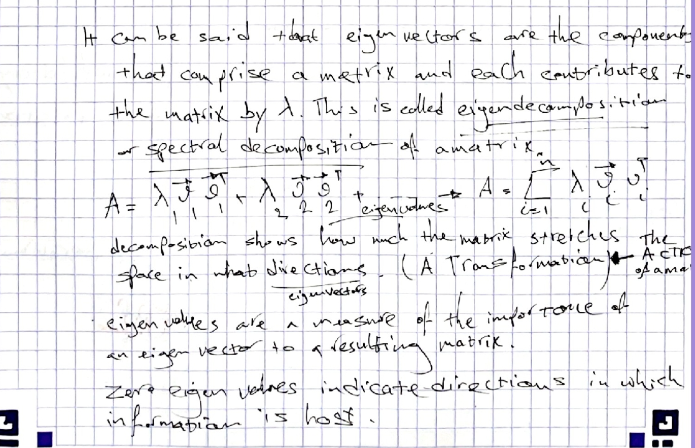
Geometrically, this means that when A is applied to v, the result is a vector pointing in the same (or opposite) direction as v, but possibly scaled by λ.

Finding Eigenvalues

To find the eigenvalues of a matrix A:

1. Write the eigenvalue equation: Av = λv
2. Rearrange to: (A - λI)v = 0, where I is the identity matrix
3. This system has non-zero solutions v if and only if det(A - λI) = 0
4. Solve the characteristic equation: det(A - λI) = 0
5. The roots of this equation are the eigenvalues of A

Finding Eigenvectors

For each eigenvalue λ:

1. Substitute λ back into (A - λI)v = 0
2. Solve this homogeneous system to find the non-zero solutions v
3. These solutions form the eigenspace for eigenvalue λ

The dimension of the eigenspace equals the algebraic multiplicity of λ minus its geometric multiplicity (the number of linearly independent eigenvectors corresponding to λ).

Properties of Eigenvalues and Eigenvectors

1. Determinant: det(A) equals the product of all eigenvalues (counting multiplicities)

2. Trace: tr(A) (sum of diagonal elements) equals the sum of all eigenvalues

3. Similar matrices: If B = P⁻¹AP, then B has the same eigenvalues as A

4. Matrix powers: If λ is an eigenvalue of A with eigenvector v, then λᵏ is an eigenvalue of Aᵏ with the same eigenvector

5. Matrix functions: If λ is an eigenvalue of A with eigenvector v, then f(λ) is an eigenvalue of f(A) with the same eigenvector

6. Inverse: If λ ≠ 0 is an eigenvalue of A, then 1/λ is an eigenvalue of A⁻¹

7. Transpose: A and A^T have the same eigenvalues

Special Cases

1. Symmetric Matrices

For a symmetric matrix (A = A^T):

• All eigenvalues are real
• Eigenvectors corresponding to distinct eigenvalues are orthogonal
• A complete set of orthogonal eigenvectors always exists

2. Triangular Matrices

For triangular matrices (upper or lower):

• The eigenvalues are exactly the diagonal entries

3. Diagonalizable Matrices

A matrix A is diagonalizable if and only if:

• It has n linearly independent eigenvectors (where n is the dimension)
• Equivalently, the sum of the dimensions of all eigenspaces equals n

If A is diagonalizable, then:

• There exists an invertible matrix P such that P⁻¹AP = D
• D is a diagonal matrix with the eigenvalues on the diagonal
• The columns of P are the eigenvectors of A

4. Complex Eigenvalues

When working in ℝ:

• Complex eigenvalues always appear in conjugate pairs: λ = a + bi and λ* = a - bi
• If v is an eigenvector for λ = a + bi, then v* is an eigenvector for λ* = a - bi

Step-by-Step Calculation Process

Example: 2×2 Matrix

For A = $\begin{bmatrix} 3 & 8 \ 0 & 4 \end{bmatrix}$:

1. Form the characteristic equation: det(A - λI) = det($\begin{bmatrix} 3-λ & 8 \ 0 & 4-λ \end{bmatrix}$) = 0

2. Calculate the determinant: (3-λ)(4-λ) - 8×0 = 0 (3-λ)(4-λ) = 0

3. Solve for λ: λ = 3 or λ = 4

4. Find eigenvectors for λ = 3: (A - 3I)v = $\begin{bmatrix} 0 & 8 \ 0 & 1 \end{bmatrix} \begin{bmatrix} v_1 \ v_2 \end{bmatrix}$ = $\begin{bmatrix} 0 \ 0 \end{bmatrix}$

   This gives 8v₂ = 0 and v₂ = 0 With v₂ = 0, v₁ can be any non-zero value Eigenvector: v = $\begin{bmatrix} 1 \ 0 \end{bmatrix}$

5. Find eigenvectors for λ = 4: (A - 4I)v = $\begin{bmatrix} -1 & 8 \ 0 & 0 \end{bmatrix} \begin{bmatrix} v_1 \ v_2 \end{bmatrix}$ = $\begin{bmatrix} 0 \ 0 \end{bmatrix}$

   This gives -v₁ + 8v₂ = 0, so v₁ = 8v₂ With v₂ = 1, v₁ = 8 Eigenvector: v = $\begin{bmatrix} 8 \ 1 \end{bmatrix}$

Example: 3×3 Matrix

For A = $\begin{bmatrix} 1 & 0 & 1 \ 0 & 3 & 0 \ 1 & 0 & 1 \end{bmatrix}$:

1. Form the characteristic equation: det(A - λI) = det($\begin{bmatrix} 1-λ & 0 & 1 \ 0 & 3-λ & 0 \ 1 & 0 & 1-λ \end{bmatrix}$) = 0

2. Calculate the determinant (using cofactor expansion along the second column): (3-λ) × [det($\begin{bmatrix} 1-λ & 1 \ 1 & 1-λ \end{bmatrix}$)] = 0 (3-λ) × [(1-λ)(1-λ) - 1×1] = 0 (3-λ) × [(1-λ)² - 1] = 0

3. Solve for λ: (3-λ) = 0 or (1-λ)² - 1 = 0 λ = 3 or (1-λ)² = 1 λ = 3 or 1-λ = ±1 λ = 3 or λ = 0 or λ = 2

4. Find eigenvectors for each eigenvalue by solving (A - λI)v = 0

Eigenvalue Multiplicities

Algebraic Multiplicity

The power to which (λ - λᵢ) appears in the characteristic polynomial.

Geometric Multiplicity

The dimension of the eigenspace corresponding to λᵢ (i.e., the number of linearly independent eigenvectors).

For a diagonalizable matrix, the algebraic and geometric multiplicities are equal for each eigenvalue.

Diagonalization Process

To diagonalize a matrix A:

1. Find all eigenvalues λ₁, λ₂, …, λₙ of A
2. For each eigenvalue λᵢ, find a basis for its eigenspace
3. Combine these bases to form the columns of matrix P
4. The diagonal matrix is D = diag(λ₁, λ₂, …, λₙ)
5. Verify that P⁻¹AP = D

A matrix is diagonalizable if and only if it has enough linearly independent eigenvectors to form a basis for the entire space.

Applications of Eigenvalues and Eigenvectors

1. Matrix powers: A^k = PD^kP⁻¹ (where D^k is easy to compute)
2. Dynamical systems: Predicting long-term behavior
3. Principal component analysis: Finding directions of maximum variance
4. Differential equations: Solving systems of differential equations
5. Markov chains: Finding steady-state distributions

Strategies for Specific Problem Types

1. Finding Eigenvalues of Triangular or Simple Matrices

For triangular matrices, eigenvalues are the diagonal entries.

2. Handling Repeated Eigenvalues

For an eigenvalue λ with algebraic multiplicity m:

• If the geometric multiplicity equals m, proceed normally
• If the geometric multiplicity is less than m, the matrix is not diagonalizable

3. Small Matrices with Simple Patterns

Look for symmetries or special structures:

• Symmetric matrices have real eigenvalues and orthogonal eigenvectors
• Matrices with repeated rows/columns often have 0 as an eigenvalue

4. Computing Matrix Functions

For a diagonalizable matrix A = PDP⁻¹:

• A^k = PD^kP⁻¹
• e^A = Pe^DP⁻¹
• Where e^D = diag(e^λ₁, e^λ₂, …, e^λₙ)

Common Mistakes to Avoid

1. Forgetting that eigenvectors cannot be the zero vector
2. Errors in calculating det(A - λI)
3. Not checking for linear independence of eigenvectors
4. Confusing algebraic and geometric multiplicities
5. Computational errors when finding eigenvectors

Exercise Examples

Example 1: 2×2 Matrix with Complex Eigenvalues

For A = $\begin{bmatrix} 3 & 8 \ 2 & 3 \end{bmatrix}$:

1. Characteristic equation: det(A - λI) = (3-λ)(3-λ) - 8×2 = 0 (3-λ)² - 16 = 0 λ² - 6λ + 9 - 16 = 0 λ² - 6λ - 7 = 0

2. Using the quadratic formula: λ = (6 ± √(36+28))/2 = (6 ± √64)/2 = (6 ± 8)/2 λ₁ = 7, λ₂ = -1

3. Find eigenvectors for each eigenvalue

Example 2: 3×3 Matrix Diagonalization

For A = $\begin{bmatrix} 2 & 1 & 0 \ 0 & 1 & -1 \ 0 & 2 & 4 \end{bmatrix}$:

1. Find eigenvalues using det(A - λI) = 0
2. For each eigenvalue, find a basis for its eigenspace
3. Form the matrix P whose columns are these eigenvectors
4. Verify that P⁻¹AP = diag(λ₁, λ₂, λ₃)

See:

• Real Eigen Values
• Complex Eigen Values

Exercises

1. Given the matrix $A = \begin{pmatrix} -1 & -1 \ -1 & -1 \end{pmatrix}$,

   (i) for each eigenvalue of $A$, find the corresponding eigenspace;

   (ii) find, if there exist, a diagonal matrix $D$ and an invertible matrix $C$ such that $C^{-1}AC = D$;

   (iii) check that $C^{-1}AC = D$.

2. Determine the eigenvalues of $A$ in $\mathbb{R}$ where $A = \begin{pmatrix} -1 & 8 \ 0 & 4 \end{pmatrix}$

3. Determine the eigenvalues of $A$ in $\mathbb{R}$ where $A = \begin{pmatrix} 3 & 8 \ 0 & 4 \end{pmatrix}$

4. Find the eigenvalues and eigenvectors of the following linear transformations:

   • $f: \mathbb{R}^2 \to \mathbb{R}^2$ where $f(x, y) = (2x + 9y, x + 2y)$
   • $f: \mathbb{R}^3 \to \mathbb{R}^3$ where $f(x, y, z) = (4x - y - 2z, 2x + y - 2z, x - y + z)$